Take-home Exercise 3

Putting Visual Analytics into Practical Use

Author

Tasaporn Visawameteekul

Published

February 6, 2023

1. The task

In this take-home exercise, you are required to uncover the salient patterns of the resale prices of public housing property by residential towns and estates in Singapore by using appropriate analytical visualisation techniques learned in Lesson 4: Fundamentals of Visual Analytics. Students are encouraged to apply appropriate interactive techniques to enhance user and data discovery experiences.

For the purpose of this study, the focus should be on 3-ROOM, 4-ROOM and 5-ROOM types. You can choose to focus on either one housing type or multiple housing types. The study period should be on 2022.

The write-up of the take-home exercise should include but not limited to the followings:

Describe the selection and designed consideration of the analytical data visualisation used. The discussion should limit to not more than 150 words each.
A reproducible description of the procedures used to prepare the analytical visualisation. Please refer to the peer submission I shared.
A write-up of not more than 100 words to discuss the patterns reveal by each analytical visualisation prepared.

2. Data

The original dataset ’Resale flat princes based on registration date from Jan-2017 onwards’ was obtained from Data.gov.sg. This dataset provides information on all resale HDB flat transactions from 2017 to 2023. The notable features in this dataset are as follows:
i) town: the town of the associated HDB flat
ii) flat_type: the type of flat of the associated HDB flat. In Singapore, there are 1-room flats up to 5-room flats, as well as executive flats, which are slightly bigger than 5-room flats. (The remaining flat type: Multi-generational flats, are few and far between)
iii) block: the block of the associated HDB flat
iv) street: the street of the associated HDB flat
v) storey_range: the storey range of the associated HDB flat. In this dataset, the storey range is given in a range of 3 (e.g. 10 to 12 , which means the flat is based on the 10th to 12th storey).
vi) floor_area_sqm: the floor area of the associated HDB flat in square meters
vii) remaining_lease: the remaining lease of the associated HDB flat in months and years
viii) resale_price: the resale price of the assocaited HDB flat

3. Design Consideration

4. Step to create plot in R

1. Installing and loading the required libraries

The code chunk below is used to install and load the required packages onto RStudio.

tidyverse : A collection of core packages designed for data science, used extensively for data preparation and wrangling. (readr, ggplot2, dplyr, purrr, tidyr, tibble)
ggstatplot: an extension of ggplot2 package for creating graphics with details from statistical tests included in the plots themselves and targeted primarily at behavioral sciences community to provide a one-line code to produce information-rich plots.
psych: A general purpose toolbox for personality, psychometric theory and experimental psychology. Functions are primarily for multivariate analysis and scale construction using factor analysis, principal component analysis, cluster analysis and reliability analysis, although others provide basic descriptive statistics.
lubridate: Provides tools that make it easier to parse and manipulate dates. These tools are grouped below by common purpose.
ggrepel: This package contains extra geoms for ggplot2.

Code

packages = c('tidyverse', 'ggstatsplot', 'psych', 'lubridate', 'ggrepel', 'plotly')
for(p in packages){
  if(!require(p,character.only = T)){
    install.packages(p)
  }
  library(p,character.only = T)
}

2. Importing the dataset

The source file is in csv format, hence read_csv of readr package is used to import the dataset. From the result below, we will see that our original data has 146,215 rows with 11 columns ( 8 categorical fields and 3 numeric fields).

Code

Resale_raw <- read_csv("Data/resale-flat-prices-based-on-registration-date-from-jan-2017-onwards.csv")
glimpse(Resale_raw)

Rows: 146,215
Columns: 11
$ month               <chr> "2017-01", "2017-01", "2017-01", "2017-01", "2017-…
$ town                <chr> "ANG MO KIO", "ANG MO KIO", "ANG MO KIO", "ANG MO …
$ flat_type           <chr> "2 ROOM", "3 ROOM", "3 ROOM", "3 ROOM", "3 ROOM", …
$ block               <chr> "406", "108", "602", "465", "601", "150", "447", "…
$ street_name         <chr> "ANG MO KIO AVE 10", "ANG MO KIO AVE 4", "ANG MO K…
$ storey_range        <chr> "10 TO 12", "01 TO 03", "01 TO 03", "04 TO 06", "0…
$ floor_area_sqm      <dbl> 44, 67, 67, 68, 67, 68, 68, 67, 68, 67, 68, 67, 67…
$ flat_model          <chr> "Improved", "New Generation", "New Generation", "N…
$ lease_commence_date <dbl> 1979, 1978, 1980, 1980, 1980, 1981, 1979, 1976, 19…
$ remaining_lease     <chr> "61 years 04 months", "60 years 07 months", "62 ye…
$ resale_price        <dbl> 232000, 250000, 262000, 265000, 265000, 275000, 28…

Use head command to see the first 5 rows of the data.

Code

head(Resale_raw,5)

# A tibble: 5 × 11
  month   town     flat_…¹ block stree…² store…³ floor…⁴ flat_…⁵ lease…⁶ remai…⁷
  <chr>   <chr>    <chr>   <chr> <chr>   <chr>     <dbl> <chr>     <dbl> <chr>  
1 2017-01 ANG MO … 2 ROOM  406   ANG MO… 10 TO …      44 Improv…    1979 61 yea…
2 2017-01 ANG MO … 3 ROOM  108   ANG MO… 01 TO …      67 New Ge…    1978 60 yea…
3 2017-01 ANG MO … 3 ROOM  602   ANG MO… 01 TO …      67 New Ge…    1980 62 yea…
4 2017-01 ANG MO … 3 ROOM  465   ANG MO… 04 TO …      68 New Ge…    1980 62 yea…
5 2017-01 ANG MO … 3 ROOM  601   ANG MO… 01 TO …      67 New Ge…    1980 62 yea…
# … with 1 more variable: resale_price <dbl>, and abbreviated variable names
#   ¹flat_type, ²street_name, ³storey_range, ⁴floor_area_sqm, ⁵flat_model,
#   ⁶lease_commence_date, ⁷remaining_lease

3. Wrangling data

3.1 Select interested fields

Code

Resale <-Resale_raw %>%
  select("month", "town", "flat_type", "storey_range", "floor_area_sqm", "lease_commence_date", "remaining_lease", "resale_price")

3.2 Filter the analyzing year of 2022

Separating column month using separate(). Filter only Year of 2022.

Code

Resale <-Resale %>%
  mutate(quarter = quarter(ym(month)))

Code

Resale <-Resale %>%
  separate(`month`, into = c("Year", "Month"), sep = "-") %>% 
  filter(Year == "2022")

3.3 Filter flat types 3-Room, 4-Room, 5-Room

Code

Resale <- Resale %>% 
  filter(flat_type %in% c("3 ROOM","4 ROOM", "5 ROOM"))

3.4 Change format of price to represent in kSGD

Code

Resale <- Resale %>%
  mutate(resale_price=resale_price/1000) %>% 
  rename('resale_price_kSGD' = 'resale_price')

3.5 Change format of remaining lease to represent in years

Code

# library(stringr)
Resale <-Resale %>%
  separate(`remaining_lease`, into = "remaining_lease", sep = " years") %>% 
  mutate(remaining_lease = as.numeric(remaining_lease))

Here, we can see that our data now only has 24,374 rows left after filter year and flat type.

Code

Resale

# A tibble: 24,374 × 10
   Year  Month town      flat_…¹ store…² floor…³ lease…⁴ remai…⁵ resal…⁶ quarter
   <chr> <chr> <chr>     <chr>   <chr>     <dbl>   <dbl>   <dbl>   <dbl>   <int>
 1 2022  01    ANG MO K… 3 ROOM  07 TO …      73    1977      54     358       1
 2 2022  01    ANG MO K… 3 ROOM  07 TO …      67    1978      55     355       1
 3 2022  01    ANG MO K… 3 ROOM  07 TO …      68    1981      58     338       1
 4 2022  01    ANG MO K… 3 ROOM  07 TO …      82    1980      57     420       1
 5 2022  01    ANG MO K… 3 ROOM  04 TO …      67    1980      57     328       1
 6 2022  01    ANG MO K… 3 ROOM  01 TO …      83    1979      56     360       1
 7 2022  01    ANG MO K… 3 ROOM  01 TO …      67    1980      57     300       1
 8 2022  01    ANG MO K… 3 ROOM  04 TO …      67    1979      56     333       1
 9 2022  01    ANG MO K… 3 ROOM  04 TO …      67    1979      56     386       1
10 2022  01    ANG MO K… 3 ROOM  10 TO …      67    1980      57     330       1
# … with 24,364 more rows, and abbreviated variable names ¹flat_type,
#   ²storey_range, ³floor_area_sqm, ⁴lease_commence_date, ⁵remaining_lease,
#   ⁶resale_price_kSGD

4. Exploratory Data Analysis

Using the describe() function, you can get a sense-check of the data and see if there were any errors in the feature engineering. These are the summary statistics that were observed:

Resale Price — The prices of the flats range between $200K to $1,418K with a mean of $536K
Floor Area — The sizes of the flats range between 51sqm to 159sqm, with a mean of 94.07sqm
Remaining Lease — The lease commence date of the flats range between 43 years to 96 years

Code

describe(Resale)

                    vars     n    mean     sd median trimmed    mad  min  max
Year*                  1 24374    1.00   0.00      1    1.00   0.00    1    1
Month*                 2 24374    6.50   3.44      7    6.51   4.45    1   12
town*                  3 24374   15.12   7.88     17   15.47   8.90    1   26
flat_type*             4 24374    2.02   0.73      2    2.02   1.48    1    3
storey_range*          5 24374    3.36   2.09      3    3.08   1.48    1   17
floor_area_sqm         6 24374   94.07  19.32     93   93.99  25.20   51  159
lease_commence_date    7 24374 1997.46  14.98   1998 1997.83  20.76 1967 2019
remaining_lease        8 24374   74.06  15.02     74   74.46  20.76   43   96
resale_price_kSGD      9 24374  536.39 157.99    515  520.46 133.43  200 1418
quarter               10 24374    2.50   1.10      3    2.50   1.48    1    4
                    range  skew kurtosis   se
Year*                   0   NaN      NaN 0.00
Month*                 11 -0.02    -1.19 0.02
town*                  25 -0.31    -1.16 0.05
flat_type*              2 -0.02    -1.13 0.00
storey_range*          16  1.66     4.36 0.01
floor_area_sqm        108 -0.06    -0.85 0.12
lease_commence_date    52 -0.03    -1.33 0.10
remaining_lease        53 -0.04    -1.32 0.10
resale_price_kSGD    1218  1.09     1.81 1.01
quarter                 3 -0.02    -1.33 0.01

5. Visualizations

5.1 Plotting histogram of resale price

Findings:

Right-skewed distribtion plot has a mean of $527k resale price.
The mode (peak) for resale price hover around $420000 mark having a count of nearing 750 transactions.
The right tail is longer.
This gives a distribution pattern of frequency on transaction prices generally falls under.

Code

gghistostats(
  data = Resale,
  x = 'resale_price_kSGD',
  type = "bayes",
  test.value = 60,
  xlab = "resale_price (kSGD)" ) +
  ggtitle("What is the overall Resale price distribution?")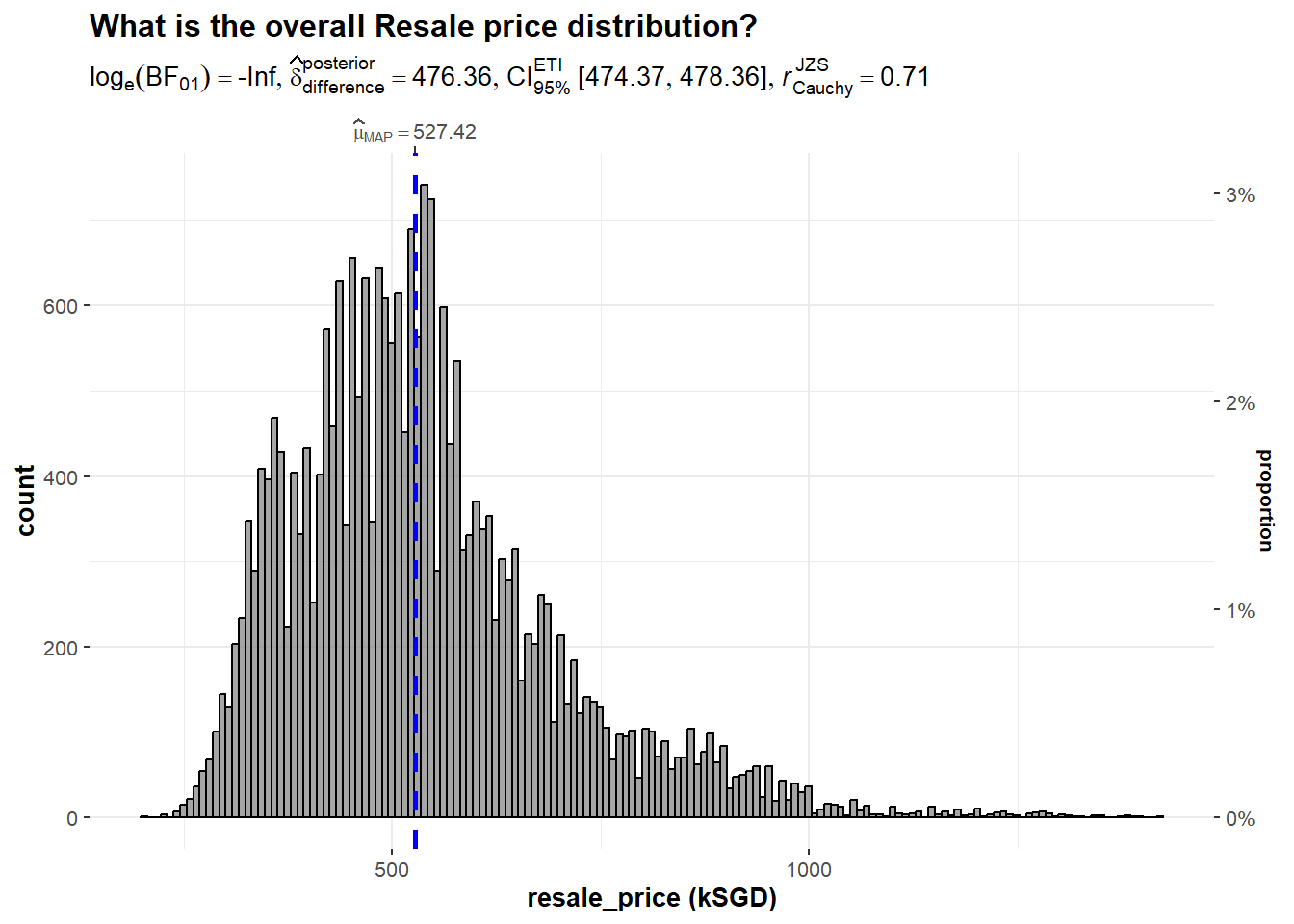

5.2 Plotting histogram of floor area

Code

gghistostats(
  data = Resale,
  x = 'floor_area_sqm',
  type = "bayes",
  test.value = 60,
  xlab = "floor_area_sqm" ) +
  ggtitle("What is the overall floor area distribution?")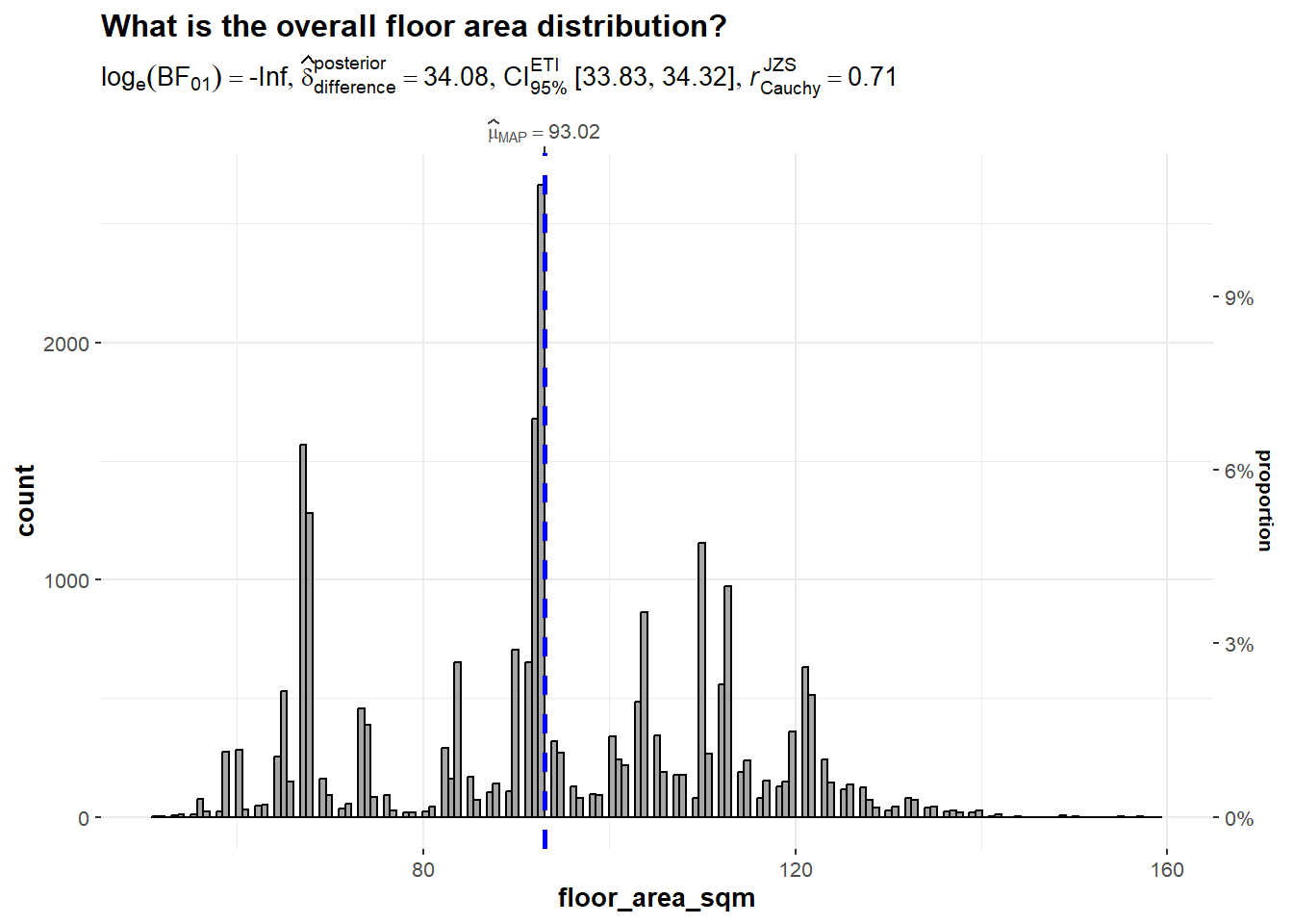

5.3 Two sample mean test on resale price between flat types

Code

ggbetweenstats(
  data = Resale,
  x = 'flat_type', 
  y = 'resale_price_kSGD',
  type = "np",
  messages = FALSE) +
  ggtitle("What is the difference in resale price between different types of flats?")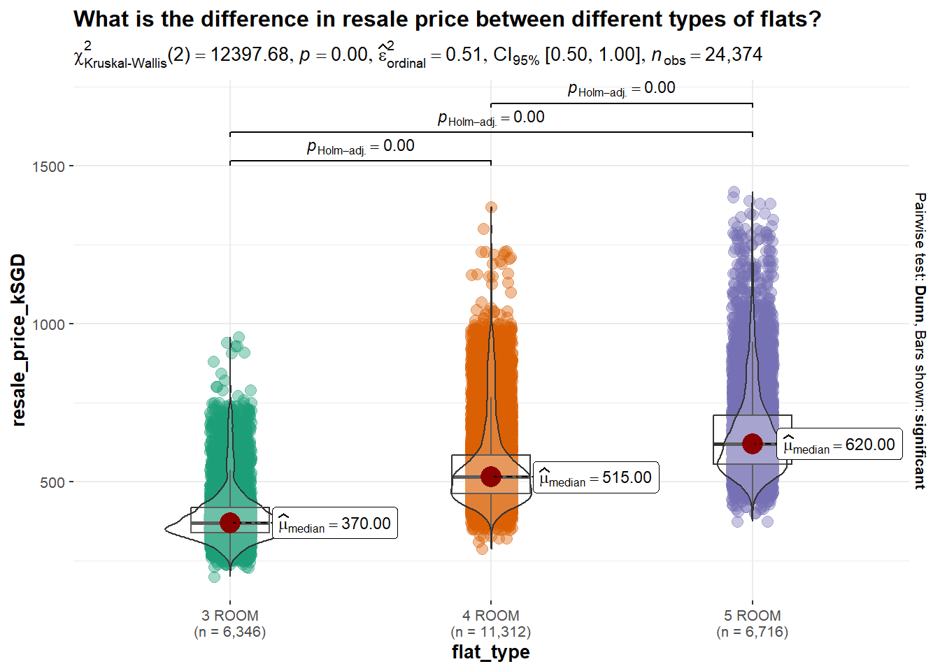

5.4 Box plot of resale price by flat types

A boxplot was also used to understand the relationship between the flat types and resale prices. It can be seen that there are quite a number of outliers in all 3 flat types.

Code

p<-ggplot(Resale, aes(x=flat_type, y=resale_price_kSGD, fill=flat_type)) +
  geom_boxplot() +
  stat_summary(fun.y=mean, geom="point", color="red") +
  theme(legend.position="none") +
  ggtitle("Boxplot of resale price by flat type")
# Remove legend
#| fig-height: 12
#| fig-width: 12
p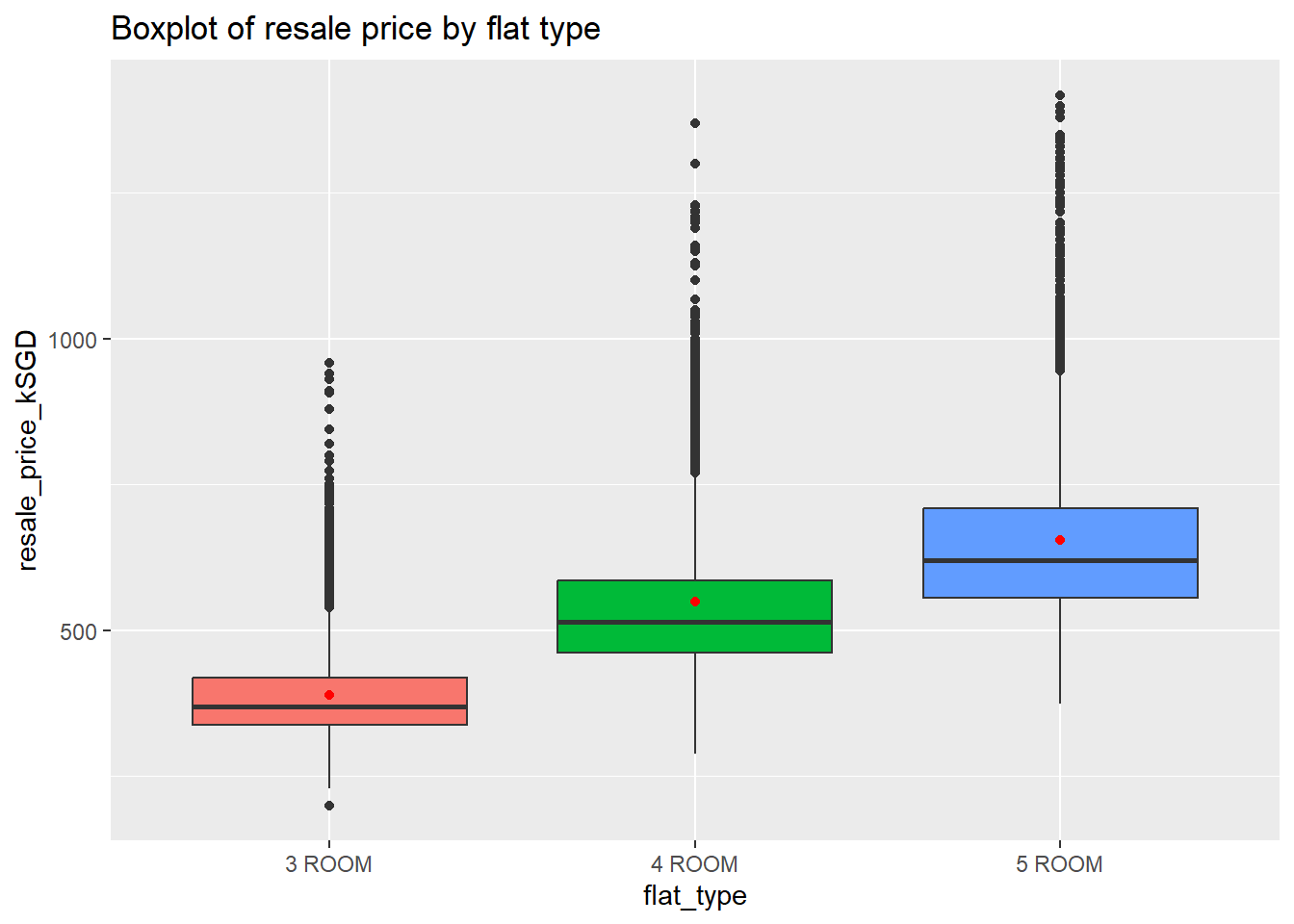

5.5 Box plot of resale price by town

Code

Resale %>%
  mutate(class = fct_reorder(town, resale_price_kSGD, .fun='mean')) %>%
  ggplot( aes(x=reorder(town, resale_price_kSGD), y=resale_price_kSGD)) +
  geom_boxplot() +
  stat_summary(fun.y=mean, geom="point", color="red") +
  theme(legend.position="none") +
  theme(axis.text.x = element_text(angle = 90, vjust = 0.5, hjust=1)) +
  ggtitle("Boxplot of resale price by town")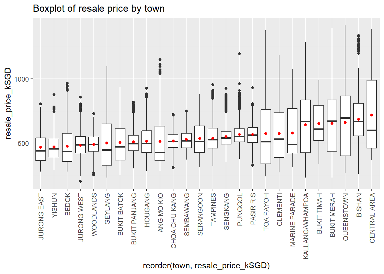

5.6 HDB resale prices in 2022 by town

Code

Resale %>% 
  group_by(flat_type) %>% 
  # Extract quarter and price per sqm
  mutate(price_per_sqm = resale_price_kSGD/floor_area_sqm) %>%
  ggplot(mapping = aes(x = town, y = price_per_sqm)) +
  # Make grouped boxplot
  geom_boxplot(aes(fill = as.factor(flat_type)), color = "grey") +
  theme_minimal() +
  theme(legend.position = "top") +
  scale_fill_viridis_d(option = "C") +
  # Adjust lables and add title
  labs(title = "HDB resale prices in 2022 by town", y="Price per square metre (SGD)", fill = "flat_type")+
  theme(axis.text.x = element_text(angle = 90, vjust = 0.5, hjust=1))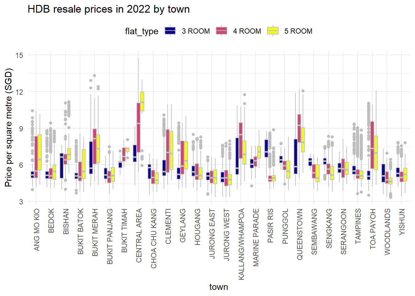

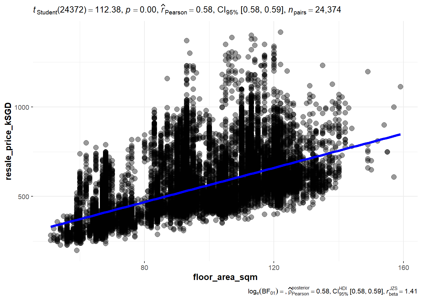
5.7 Significant Test of Correlation: ggscatterstats()

Code

ggscatterstats(
  data = Resale,
  x = floor_area_sqm,
  y = resale_price_kSGD,
  marginal = FALSE
  )

Code

p <- ggscatterstats(
  data = Resale,
  x = floor_area_sqm,
  y = resale_price_kSGD,
  marginal = FALSE,
  point.args = list(size = 0.5, alpha = 0.1, stroke = 0, color = "red"),
  smooth.line.args = list(linewidth = 0.5, color = "blue", method = "lm", formula = y ~
    x)
  )
      
p1 <- p +  facet_wrap (~ town, nrow = 6, ncol = 6) + 
            xlab("floor area") +
            scale_y_continuous(breaks = c(0,3000,6000,9000,12000), name = "Resale price(kSGD)")

ggplotly(p1)

5.8

Code

ggplot(data = Resale, mapping = aes(y=town, fill=flat_type)) +
  theme_minimal() +
  geom_bar(position = "fill") +
  scale_fill_viridis_d(option = "C") +
  labs(title = "Flat type proportion by town", fill = "Flat type", 
       x = "Count", y = "")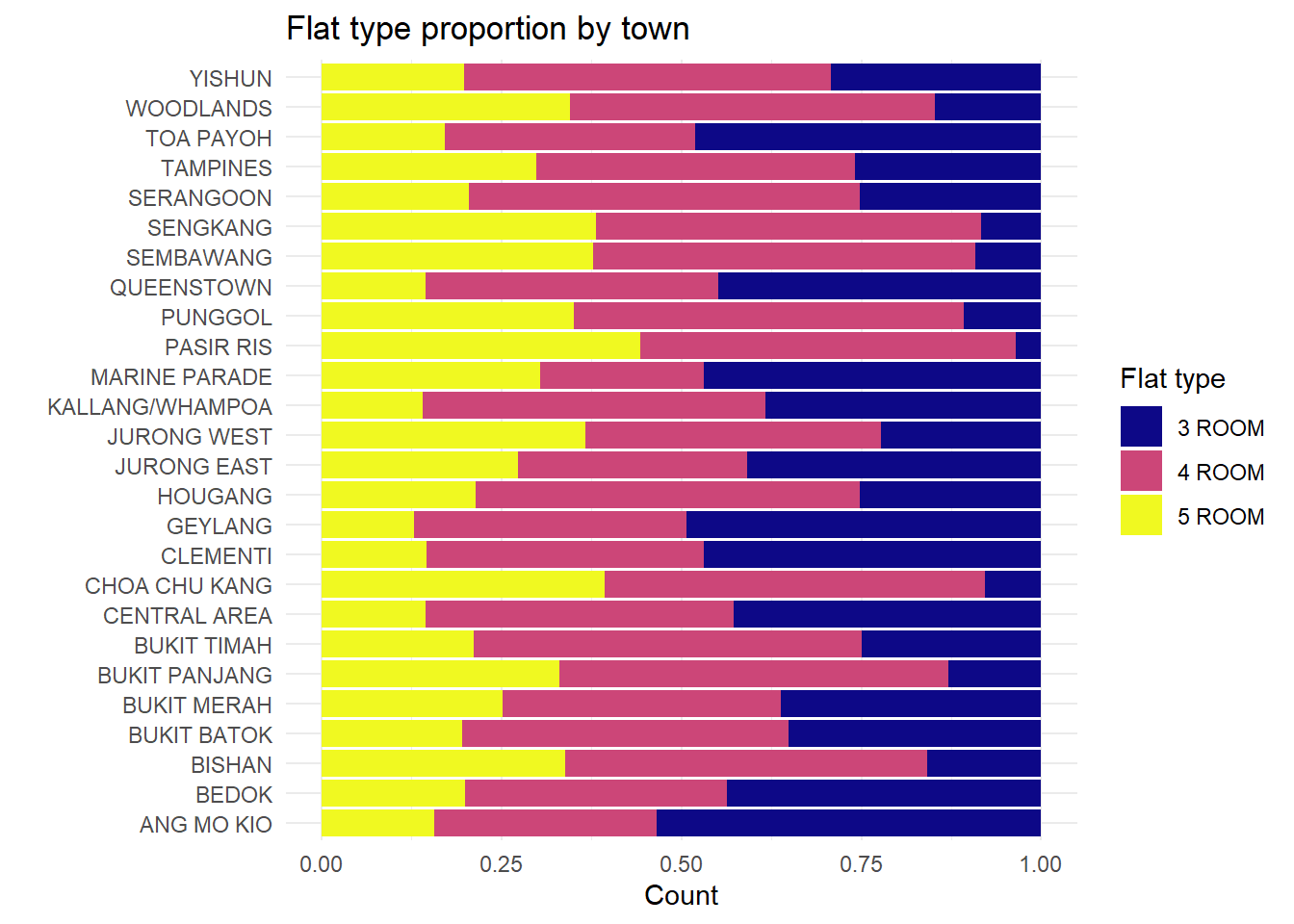

5.9 How have prices fluctuated in 2022 for different flat types?

We display a quarterly boxplot to illustrate the price trend over time. As room count increases, the average price per square meter drops. There are numerous outliers with extremely high prices per square meter in 3, 4, and 5 ROOM. The type of flat with the highest.

Code

Resale %>% 
  group_by(flat_type) %>% 
  # Extract quarter and price per sqm
  mutate(price_per_sqm = resale_price_kSGD/floor_area_sqm) %>%
  ggplot(mapping = aes(x = flat_type, y = price_per_sqm)) +
  # Make grouped boxplot
  geom_boxplot(aes(fill = as.factor(quarter)), color = "black") +
  theme_minimal() +
  theme(legend.position = "top") +
  scale_fill_viridis_d(option = "C") +
  # Adjust lables and add title
  labs(title = "HDB resale prices in 2022 by flat type", y="Price per square metre (SGD)", fill = "Quarter")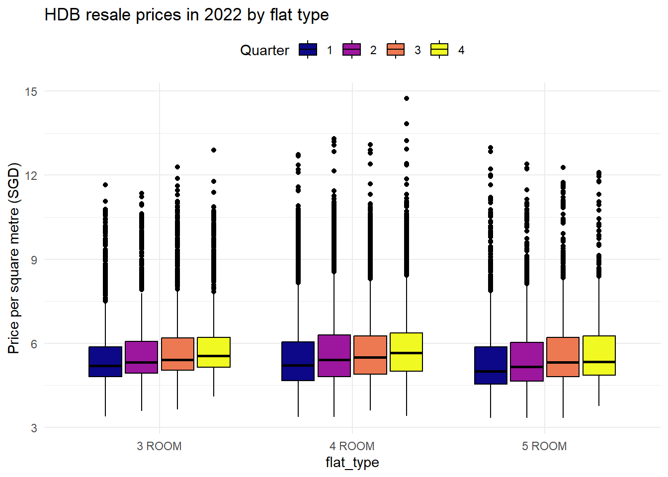

5.10 Resale flat type by town

Code

Resale %>% 
  group_by(town) %>% 
  # Calculate housing age
  mutate(housing_age = 2023 - lease_commence_date) %>% 
  summarise(average_price = mean(resale_price_kSGD), average_housing_age = mean(housing_age), average_area = mean(floor_area_sqm)) %>% 
  ggplot(mapping = aes(x=average_housing_age, y=average_price)) +
  geom_count(aes(color = average_area), alpha = 0.6) +
  # Change size of count points
  scale_size_area(max_size = 10) +
  # Add lables next to count points
  geom_text_repel(aes(label = town),size = 2.7) +
  scale_y_continuous( limits = c(400, 800)) +
  theme_minimal() +
  theme(legend.position = "top") +
  scale_color_viridis_c(option = "C")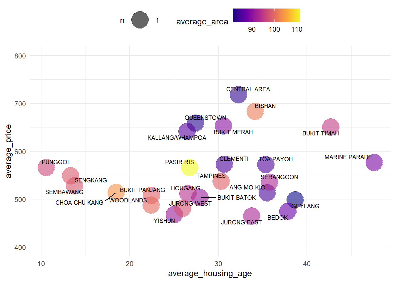

5. Reference

https://r4ds.had.co.nz/index.html

https://r-graph-gallery.com/267-reorder-a-variable-in-ggplot2.html

https://wangjing.city/wp-content/uploads/2021/05/Looking-into-Singapore-Resale-Flats-Market.html

https://towardsdatascience.com/understanding-and-predicting-resale-hdb-flat-prices-in-singapore-1853ec7069b0

https://rpubs.com/chunwey/LinearR2

https://www.linkedin.com/pulse/data-analytics-understanding-resale-prices-hdb-houses-bannister/?trk=read_related_article-card_title

https://wangjing.city/portfolio/looking-into-singapore-resale-flats-market/

https://stackoverflow.com/questions/1330989/rotating-and-spacing-axis-labels-in-ggplot2

http://www.sthda.com/english/wiki/ggplot2-axis-ticks-a-guide-to-customize-tick-marks-and-labels